Model description
Quick Overview
This section provides a summary of the main processes, equations, and configuration parameters in AeoLiS. For more information, refer to the detailed sections linked in the text (or scroll further down this page).
For guidance on setting up an AeoLiS model, see the model in- & output guide. The main configuration file (default: aeolis.txt) is the basis of the model setup and contains all parameter settings and process-flags, and serves as the central reference for other input files. The computational domain is constructed using x- and y-coordinates (xgrid_file, ygrid_file) alongside the initial bed elevation (bed_file). External environmental forcing is defined through continuous time series of wind (wind_file), water levels (tide_file), and waves (wave_file).
The simulation advances sequentially through time steps, repeating all activated processes and continuously updating the morphological model state. The simulation duration runs from a defined start time (tstart) to an end time (tstop), both specified in seconds relative to a designated reference date (refdate). A typical internal time step (dt) is 3600 seconds (1 hour). As the model progresses, it exports user-defined variables (output_vars) to a NetCDF file (default: aeolis.nc, defined by output_file) at customized intervals (output_times).
Note
In the AeoLiS source code, all model parameters are stored in two dictionaries for BMI-compatibility. All parameters defined on the computational domain, i.e., with dimension (ny,``nx``), are stored in the s-dictionary (e.g., s['x']), while all single parameters are stored in the p-dictionary (e.g., p['dt']).
Sediment Transport
Detailed section: sediment transport section.
Aeolian sediment transport is the core of the AeoLiS model. It is computed using a two-dimensional advection scheme, simplified here for one-dimensional transport of a single sediment fraction:
The right-hand side of the advection equation represents the net entrainment (pickup); the difference between erosion \(E\) and deposition \(D\) [\(\mathrm{kg/m^2/s}\)]. The saturated sediment concentration \(c_{\mathrm{sat}}\) (Cu) [\(\mathrm{kg/m^2}\)] defines the transport capacity, while \(c\) (Ct) [\(\mathrm{kg/m^2}\)] is the instantaneous concentration in the air. Transport is activated in the configuration file using process_transport. This net entrainment is governed by the adaptation timescale \(T\) (T) [\(\mathrm{s}\)], which determines how quickly the concentration reaches equilibrium. To allow sediment to actually erode from or deposit to the bed, process_bedupdate must be enabled.
Solving this advection equation is one of the most computationally expensive parts of the model. You can choose different numerical approaches using the solver keyword. For detailed guidance on these options, see the solver guide.
Several methods are available to compute the saturated sediment concentration (method_transport). The equation by [Bagnold, 1937] (bagnold) is the default:
The sediment velocity \(u_{\mathrm{sed}}\) (u, us, un) [\(\mathrm{m/s}\)] is determined by the method_grainspeed parameter. It can either be set equal to the governing wind speed (windspeed) or calculated using a saltation model (e.g., duran). For more information on grain speed computations, see the sediment velocity section.
Note
For all vector variables (like uw, ustar, tau, u, q), the subscripts s and n (e.g., uws, uwn) indicate the cross-shore and longshore directions, respectively, and the name without a subscript represents the overall magnitude.
AeoLiS supports the inclusion of multiple sediment fractions (grain_size, grain_dist) across multiple vertical layers (nlayers). This allows for the simulation of sediment sorting, mixing, and armoring. More details are provided in the multi-fraction sediment transport section.
Enabling process_bedinteraction incorporates a bed interaction parameter into the advection equation. For more information, see the bed interaction approach section.
Wind and Shear Velocity
Detailed section: Wind and Shear Velocity
The shear velocity \(u_*\) (ustar) [\(\mathrm{m/s}\)] acts as the primary driver of sediment transport. It is initially computed for a flat bed using the Prandtl-Von Kármán Law of the Wall, based on the wind velocity \(u_w\) (uw) [\(\mathrm{m/s}\)] at a given elevation. Wind conditions are provided via the wind_file and the computation is enabled via process_wind.
Topography can steer the wind, causing perturbations in the shear stress \(\tau\) (tau) [\(\mathrm{N/m^2}\)], where \(\tau = \rho_a u_*^2\):
This steering process can be activated using the process_shear keyword. Different methods are available to compute these shear perturbations, which can be selected through method_shear. More information on these computations is given in the topographic steering section.
The presence of vegetation can also reduce the effective shear stress. For more information, see the vegetation documentation.
Shear Velocity Threshold
Detailed section: Shear Velocity Threshold
Where shear velocity drives transport, the threshold velocity \(u_{\mathrm{th}}\) (uth) [\(\mathrm{m/s}\)] serves as a supply-limiter. It acts as a collective parameter for all supply-limiting processes, scaling the base threshold \(u_{\mathrm{*th,0}}\) (uth0) [\(\mathrm{m/s}\)] by various environmental factors. Threshold calculations are enabled via process_threshold.
The base threshold \(u_{\mathrm{* th, 0}}\) [\(\mathrm{m/s}\)] is computed based on the local grain size [\(\mathrm{m}\)] and density [\(\mathrm{kg/m^3}\)] (activated via th_grainsize). This base value is then scaled by supply-limiting factors depending on the enabled model processes. The influence of surface moisture (\(f_{\mathrm{M}}\)) [\(\mathrm{-}\)] is activated via th_moisture, while sheltering by non-erodible roughness elements (\(f_{\mathrm{R}}\)) [\(\mathrm{-}\)] is configured via th_sheltering. The restricting effect of a non-erodible layer can be included using th_nelayer.
Vegetation
Detailed section: Vegetation
Vegetation plays a key role in the development of dunes. The simulation of vegetation growth and spreading, along with the subsequent reduction in shear stress, can be enabled via process_vegetation. The specific vegetation formulation is selected using method_vegetation (duran for the original implementation, or grass for the newer framework by ).
In the original description, the vegetation density \(\rho_{\mathrm{veg}}\) (rhoveg) [\(\mathrm{-}\)] is computed based on the current vegetation height \(h_{\mathrm{veg}}\) (hveg) [\(\mathrm{m}\)] relative to the maximum attainable height \(H_{\mathrm{max}}\) (hveg_max or Hveg) [\(\mathrm{m}\)]:
This density determines the magnitude of the shear stress reduction acting on the sand bed, which relies on a vegetation-related roughness parameter \(\Gamma\) (gamma_vegshear) [\(\mathrm{-}\)] and the basal cover \(\rho_{\mathrm{veg}}\) (rhoveg) [\(\mathrm{-}\)]:
The vertical development of the vegetation over time is described by:
This growth is governed by the intrinsic vertical growth rate \(V_{\mathrm{ver}}\) (V_ver) [\(\mathrm{m/s}\)] and the plant’s sensitivity to sediment burial or erosion \(\gamma_{\mathrm{veg}}\) (veg_gamma) [\(\mathrm{-}\)].
Hydrodynamics and Surface Moisture
Detailed section: Hydrodynamics and Surface Moisture
Water levels, wave runup, and groundwater can wet the beach, temporarily increasing the shear velocity threshold and mixing sediment fractions. The model reads input water levels (tide_file) and wave heights (wave_file), which are activated via process_tide and process_wave.
The input water level is first projected onto the domain to establish the Still Water Level (SWL) [\(\mathrm{m}\)]. If wave runup is enabled (process_runup), the runup height (R) [\(\mathrm{m}\)] is computed and added to form the Total Water Level (TWL) [\(\mathrm{m}\)], where TWL = SWL + R. The local water surface elevation (zs) [\(\mathrm{m}\)] is then determined as the maximum of the bed level (zb) [\(\mathrm{m}\)] and the TWL, from which the actual water depth (hw) [\(\mathrm{m}\)] is derived. Spatial masks (tide_mask, wave_mask, runup_mask) can be applied to restrict or modify where these hydrodynamics act.
Inundation wets the bed, increasing the surface moisture (moist) [\(\mathrm{-}\)]. Once the beach is exposed, infiltration and evaporation gradually dry the surface. This moisture tracking is activated via process_moist. A more advanced description of intertidal groundwater fluctuations by can also be enabled through process_groundwater. For more information on these computations, see the surface moisture section.
Furthermore, wave impacts can mix multiple sediment fractions across several bed layers down to the depth of disturbance. This mixing process is enabled via process_mixtoplayer. For more details on how waves rework the bed, see the hydraulic sediment mixing section.
Morphological Change
Detailed section: Morphological change
Gradients in aeolian sediment transport result in net erosion or deposition, causing the bed level \(z_B\) (zb) [\(\mathrm{m}\)] to change over time; \(\Delta z_B\) (dzb) [\(\mathrm{m}\)]. This morphological updating is enabled by process_bedupdate:
This change is driven directly by the net entrainment \((E - D)\) (pickup) [\(\mathrm{kg/m^2/s}\)] computed in the advection equation, scaled by the sediment density \(\rho_{\mathrm{sed}}\) (rhog) [\(\mathrm{kg/m^3}\)] and the sediment porosity \(p\) (porosity) [\(\mathrm{-}\)]. Together, the density and porosity represent the bulk density of the bed. For more detailed mechanics on this mass balance, see the morphological change section.
To redistribute sediment when the local slope becomes too steep, avalanching can be enabled through process_avalanche. This routine triggers when the bed slope exceeds the static angle of repose (theta_stat) [\(\mathrm{^\circ}\)] and relaxes the slope back to the dynamic angle of repose (theta_dyn) [\(\mathrm{^\circ}\)].

Fig. 2 Overview of the AeoLiS model structure and simulated processes.
Aeolian Sediment Transport
Calculating aeolian sediment transport is the core of the AeoLiS model.
The model is based on the approach of [de Vries et al., 2014] which is extended to compute the
spatiotemporal varying sediment availability through simulation of the
process of beach armoring. For this purpose the bed is discretized in
horizontal grid cells and in vertical bed layers (nlayers) [\(\mathrm{-}\)]. Moreover, the
grain size distribution is discretized into fractions (grain_size [\(\mathrm{m}\)], grain_dist [\(\mathrm{-}\)]). This allows the
grain size distribution to vary both horizontally and vertically. A
bed composition module is used to compute the sediment availability
for each sediment fraction individually. This model approach is a
generalization of existing model concepts, like the shear velocity
threshold and critical fetch, and therefore compatible with these
existing concepts.
Advection Equation
A 1D advection scheme is adopted in correspondence with
[de Vries et al., 2014] in which \(c\) (Ct) [\(\mathrm{kg/m^2}\)] is
the instantaneous sediment mass per unit area in transport:
Here, \(t\) (_time) [\(\mathrm{s}\)] denotes time, \(x\) (x) [\(\mathrm{m}\)] denotes the cross-shore
distance, and \(u_{\mathrm{sed}}\) (u, us, un) [\(\mathrm{m/s}\)] is the sediment velocity. \(E\) and \(D\)
[\(\mathrm{kg/m^2/s}\)] represent the erosion and deposition terms
and hence combined represent the net entrainment of sediment (pickup).
Note
Equation (10) differs from Equation 9 in [de Vries et al., 2014] as they use the saltation height \(h\) [\(\mathrm{m}\)] and the volumetric sediment concentration \(C_{\mathrm{c}}\) [\(\mathrm{kg/m^3}\)]. As \(h\) is not solved for, the presented model computes the sediment mass per unit area \(c = h C_{\mathrm{c}}\) rather than the sediment concentration \(C_{\mathrm{c}}\). For conciseness we still refer to \(c\) as the sediment concentration.
The net entrainment is determined based on a balance between the
equilibrium or saturated sediment concentration
\(c_{\mathrm{sat}}\) (Cu) [\(\mathrm{kg/m^2}\)] and the
instantaneous sediment transport concentration \(c\), and is
maximized by the available sediment in the bed \(m_{\mathrm{a}}\) (mass)
[\(\mathrm{kg/m^2}\)] according to:
\(T\) (T) [\(\mathrm{s}\)] represents an adaptation time scale that is assumed
to be equal for both erosion and deposition. A time scale of 1 second
is commonly used [de Vries et al., 2014].
Solving this advection equation is one of the most computationally expensive processes in the model. The numerical approach can be selected using the solver parameter, which provides three options: steadystate, euler_backward, and euler_forward.
Tip
The steadystate solver is the default and recommended option for most applications. It is the most thoroughly tested and fastest option available. The steady-state assumption is generally valid for aeolian transport because wind and sediment transport adjust to local conditions on a scale of seconds to minutes, which is orders of magnitude faster than the timescale of typical timesteps in the AeoLiS model (hours). For detailed guidance on configuring these numerical approaches, see the solver guide.
Saturated Sediment Transport
The equilibrium, or saturated, sediment concentration \(c_{\mathrm{sat}}\) (Cu) [\(\mathrm{kg/m^2}\)] is computed using an empirical sediment transport formulation selected via the method_transport parameter. The default formulation is based on Bagnold ([Bagnold, 1937]) via the bagnold setting:
in which \(q_{\mathrm{sat}}\) [\(\mathrm{kg/m/s}\)] is the saturated sediment transport rate representing the sediment transport capacity. \(u_*\) (ustar) [\(\mathrm{m/s}\)] is the shear velocity, and \(u_{\mathrm{th}}\) (uth) [\(\mathrm{m/s}\)] is the velocity threshold. The properties of the sediment and air are represented by a series of parameters: \(C_{\mathrm{b}}\) (Cb) [\(\mathrm{-}\)] is an empirical constant, \(\rho_{\mathrm{a}}\) (rhoa) [\(\mathrm{kg/m^3}\)] is the density of the air, and \(g\) (g) [\(\mathrm{m/s^2}\)] is the gravitational constant.
The saturated sediment concentration \(c_{\mathrm{sat}}\) is directly related to the saturated sediment transport rate \(q_{\mathrm{sat}}\) and the sediment velocity \(u_{\mathrm{sed}}\) (u) [\(\mathrm{m/s}\)] through the relationship \(q_{\mathrm{sat}} = c_{\mathrm{sat}} \cdot u_{\mathrm{sed}}\). Therefore, to obtain the mass per unit area, the transport rate is divided by the sediment velocity:
Depending on the configuration, several other formulations can be selected to compute the saturated sediment concentration, for example:
kawamura:
(14)\[c_{\mathrm{sat}} = C_{\mathrm{k}} \frac{\rho_{\mathrm{a}}}{g} \frac{\left( u_* + u_{\mathrm{th}} \right)^2 \left( u_* - u_{\mathrm{th}} \right)}{u_{\mathrm{sed}}}\]
lettau:
(15)\[c_{\mathrm{sat}} = C_{\mathrm{l}} \frac{\rho_{\mathrm{a}}}{g} \frac{u_*^2 \left( u_* - u_{\mathrm{th}} \right)}{u_{\mathrm{sed}}}\]
dk:
(16)\[c_{\mathrm{sat}} = C_{\mathrm{dk}} \frac{\rho_{\mathrm{a}}}{g} \frac{0.8 u_{\mathrm{th}} \left( u_*^2 - \left( 0.8 u_{\mathrm{th}} \right)^2 \right)}{u_{\mathrm{sed}}}\]
Sediment Transport Velocity
The horizontal sediment velocity \(u_{\mathrm{sed}}\) (u) [\(\mathrm{m/s}\)] determines the advection speed of the sediment concentration. It can be computed using different approaches selected via the method_grainspeed parameter. For detailed guidance on selecting the appropriate method and its impact on computational time and landform evolution, see this guide.
The simplest approach (windspeed) assumes the horizontal sediment velocity is equal to the wind velocity \(u_{\mathrm{w}}\) (uw) [\(\mathrm{m/s}\)]:
While this method is the fastest and most robust, it overpredicts the horizontal sediment velocity because grains in saltation move slower than the wind. Consequently, it fails to capture deposition patterns, making it suitable only for bulk transport calculations.
Predictions of the actual saltation velocity provide a more realistic description of horizontal sediment movement []. The sediment velocity can be determined from a momentum balance [] consisting of three terms: the drag force acting on the grains, the loss of momentum during grain-bed interaction (splashing), and the downhill gravity force:
where \(v_{\mathrm{eff}}\) [\(\mathrm{m/s}\)] is the effective wind velocity driving the grains, which depends on the shear velocity \(u_*\) and the threshold shear velocity \(u_{\mathrm{*th}}\). \(u_{\mathrm{f}}\) [\(\mathrm{m/s}\)] is the fluid threshold velocity (or grain settling velocity), \(\nabla z_{\mathrm{B}}\) [\(\mathrm{-}\)] is the bed slope, and \(\alpha\) [\(\mathrm{-}\)] is an effective restitution coefficient for the grain-bed interaction (e.g., \(\alpha = 0.42\) for \(d = 250\) \(\mathrm{\mu m}\)).
Note
The computed \(u_{\mathrm{sed}}\) represents the collective horizontal sediment movement, not the velocity of individual grains.
AeoLiS provides three options based on this momentum balance:
duran_full solves the full momentum balance equation (Equation (18)) numerically for each timestep. This method is computationally heavy but necessary for accurate sediment velocities on steep topography (e.g., steep blowout cliffs).
duran uses an analytical approximation of the full momentum balance. It accounts for spatial variations and slope effects by assuming slopes are relatively gentle to avoid computationally expensive numerical solving:
(19)\[u_{\mathrm{sed}} \approx \left( v_{\mathrm{eff}} - \frac{u_{\mathrm{f}}}{\sqrt{2\alpha A}} \right) \hat{e}_{\tau} - \frac{\sqrt{2\alpha} u_{\mathrm{f}}}{A} \nabla z_{\mathrm{B}}\]where \(\hat{e}_{\tau}\) is the wind direction unit vector and \(A \equiv |\hat{e}_{\tau} + 2\alpha \nabla z_{\mathrm{B}}|\). The first term points toward the wind direction, while the second is directed along the surface gradient, accounting for the competing effects of wind and gravity.
duran_uniform assumes a flat bed (\(\nabla z_{\mathrm{B}} = 0\)). The sediment velocity is spatially uniform, simplifying the equation further to:
(20)\[u_{\mathrm{sed}} = v_{\mathrm{eff}} - \frac{u_{\mathrm{f}}}{\sqrt{2\alpha}}\]
Tip
Guidance on selecting a grain speed method (see :ref:`this guide <solver-guide>` for more information)
Use
duranfor most simulations involving landform evolution where topographic steering is important.Use
duran_fullonly for simulations involving topography with very steep gradients (e.g., blowout cliffs).Use
duran_uniformfor static topography where you need realistic deposition patterns but no landform migration.Use
windspeedonly for basic, bulk transport calculations where morphodynamics are irrelevant.
Multi-fraction Sediment Transport
The formulation for the equilibrium or saturated sediment
concentration \(c_{\mathrm{sat}}\) (Equation
equilibrium-conc) is capable of dealing with variations in
grain size through the variables \(u_{\mathrm{th}}\),
\(d_{\mathrm{n}}\) and \(C\) [Bagnold, 1937]. However,
the transport formulation only describes the saturated sediment
concentration assuming a fixed grain size distribution, but does not
define how multiple fractions coexist in transport. If the saturated
sediment concentration formulation would be applied to each fraction
separately and summed up to a total transport, the total sediment
transport would increase with the number of sediment fractions. Since
this is unrealistic behavior the saturated sediment concentration
\(c_{\mathrm{sat}}\) for the different fractions should be
weighted in order to obtain a realistic total sediment
transport. Equation (11) therefore is modified to include a
weighting factor \(\hat{w}_k\) in which \(k\) represents the
sediment fraction index:
It is common to use the grain size distribution in the bed as weighting factor for the saturated sediment concentration (e.g. [Delft3D-FLOW Manual, 2014], section 11.6.4). Using the grain size distribution at the bed surface as a weighting factor assumes, in case of erosion, that all sediment at the bed surface is equally exposed to the wind.
Using the grain size distribution at the bed surface as weighting
factor in case of deposition would lead to the behavior where
deposition becomes dependent on the bed composition. Alternatively, in
case of deposition, the saturated sediment concentration can be
weighted based on the grain size distribution in the air. Due to the
nature of saltation, in which continuous interaction with the bed
forms the saltation cascade, both the grain size distribution in the
bed and in the air are likely to contribute to the interaction between
sediment fractions. The ratio between both contributions in the model
is determined by a bed interaction parameter \(\zeta\) (bi).
Note
The bed interaction parameter (bi) described here is currently distinct from the recently introduced bed-interaction factor (zeta). While conceptually similar, they serve different purposes:
bi: A static variable that weights the contribution of the bed composition (sand in the bed) versus the airborne composition (sand already in transport) when computing the transport rate for multiple sediment fractions.zeta: A dynamically computed factor based on surface properties that decouples the air and bed. It determines the extent to which transport is governed by bed conditions (supply-limited) versus airborne conditions (wind-driven capacity) (see this section).
Future updates should aim to consolidate these two parameters.
The weighting of erosion and deposition of individual fractions is computed according to:
in which \(k\) represents the sediment fraction index, \(n_{\mathrm{k}}\) the total number of sediment fractions, \(w_k\) is the unnormalized weighting factor for fraction \(k\), \(\hat{w}_k\) is its normalized counterpart, \(w^{\mathrm{air}}_k\) and \(w^{\mathrm{bed}}_k\) are the weighting factors based on the grain size distribution in the air and bed respectively and \(\hat{S}_k\) is the effective sediment saturation of the air. The weighting factors based on the grain size distribution in the air and the bed are computed using mass ratios:
The sum of the ratio \(w^{\mathrm{air}}_k\) over the fractions
denotes the degree of saturation of the air column for fraction
\(k\). The degree of saturation determines if erosion of a fraction may
occur. Also in saturated situations erosion of a sediment fraction can
occur due to an exchange of momentum between sediment fractions, which
is represented by the bed interaction parameter \(\zeta\) (bi). The effective
degree of saturation is therefore also influenced by the bed
interaction parameter and defined as:
When the effective saturation is greater than or equal to unity the air is (over)saturated and no erosion will occur. The grain size distribution in the bed is consequently less relevant and the second term in Equation (23) is thus minimized and zero in case \(\zeta = 0\). In case the effective saturation is less than unity erosion may occur and the grain size distribution of the bed also contributes to the weighting over the sediment fractions. The weighting factors for erosion are then composed from both the grain size distribution in the air and the grain size distribution at the bed surface. Finally, the resulting weighting factors are normalized to sum to unity over all fractions (\(\hat{w}_k\)).
The composition of weighting factors for erosion is based on the saturation of the air column. The non-saturated fraction determines the potential erosion of the bed. Therefore the non-saturated fraction can be used to scale the grain size distribution in the bed in order to combine it with the grain size distribution in the air according to Equation (23). The non-saturated fraction of the air column that can be used for scaling is therefore \(1 - \hat{S}_k\).
For example, if bed interaction is disabled (\(\zeta = 0\)) and the air is 70% saturated, then the grain size distribution in the air contributes 70% to the weighting factors for erosion, while the grain size distribution in the bed contributes the other 30% (Figure Fig. 3, upper left panel). In case of (over)saturation the grain size distribution in transport contributes 100% to the weighting factors and the grain size distribution in the bed is of no influence. Transport progresses in downwind direction without interaction with the bed.

Fig. 3 Contributions of the grain size distribution in the bed and in the air to the weighting factors \(\hat{w}_k\) for the equilibrium sediment concentration in Equation (21) for different values of the bed interaction parameter.
To allow for bed interaction in saturated situations in which no net erosion can occur, the bed interaction parameter \(\zeta\) is used (Figure Fig. 3). The bed interaction parameter can take values between 0.0 and 1.0 in which the weighting factors for the equilibrium or saturated sediment concentration in an (over)saturated situation are fully determined by the grain size distribution in the bed or in the air respectively. A bed interaction value of 0.2 represents the situation in which the grain size distribution at the bed surface contributes 20% to the weighting of the saturated sediment concentration over the fractions. In the example situation where the air is 70% saturated such value for the bed interaction parameter would lead to weighting factors that are constituted for \(70\% \cdot (100\% - 20\%) = 56\%\) based on the grain size distribution in the air and for the other 44% based on the grain size distribution at the bed surface (Figure Fig. 3, upper right panel).
The parameterization of the exchange of momentum between sediment
fractions is an aspect of saltation that is still poorly
understood. Therefore calibration of the bed interaction parameter
\(\zeta\) is necessary. The model parameters in Equation
equilibrium-conc can be chosen in accordance with the
assumptions underlying multi-fraction sediment transport. \(C\) should
be set to 1.5 as each individual sediment fraction is well-sorted,
\(d_{\mathrm{n}}\) should be chosen equal to \(D_{\mathrm{n}}\) as the
grain size dependency is implemented through
\(u_{\mathrm{th}}\). \(u_{\mathrm{th}}\) typically varies between 1 and 6
m/s for sand.
Sediment Sorting and Beach Armoring
Since the equilibrium or saturated sediment concentration \(c_{\mathrm{sat},k}\) is weighted over multiple sediment fractions in the extended advection model, also the instantaneous sediment concentration \(c_k\) is computed for each sediment fraction individually. Consequently, grain size distributions may vary over the model domain and in time. These variations are thereby not limited to the horizontal, but may also vary over the vertical since fine sediment may be deposited on top of coarse sediment or, reversely, fines may be eroded from the bed surface leaving coarse sediment to reside on top of the original mixed sediment. In order to allow the model to simulate the processes of sediment sorting and beach armoring the bed is discretized in horizontal grid cells and vertical bed layers (2DV; Figure Fig. 4).
The discretization of the bed consists of a minimum of three vertical bed layers with a constant thickness and an unlimited number of horizontal grid cells. The top layer is the bed surface layer and is the only layer that interacts with the wind and hence determines the spatiotemporal varying sediment availability and the contribution of the grain size distribution in the bed to the weighting of the saturated sediment concentration. One or more bed composition layers are located underneath the bed surface layer and form the upper part of the erodible bed. The bottom layer is the base layer and contains an infinite amount of erodible sediment according to the initial grain size distribution. The base layer cannot be eroded, but can supply sediment to the other layers.
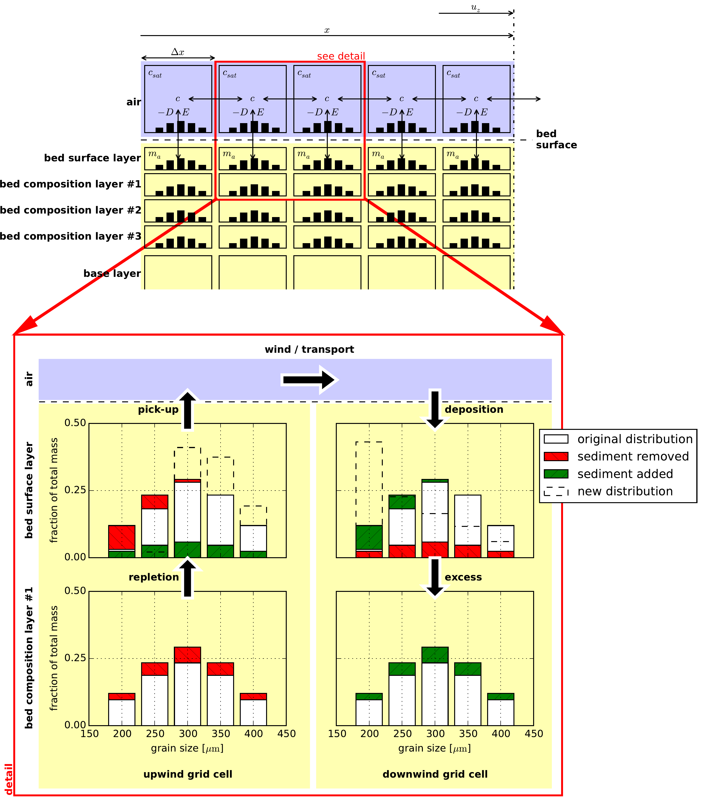
Fig. 4 Schematic of bed composition discretisation and advection scheme. Horizontal exchange of sediment may occur solely through the air that interacts with the bed surface layer. The detail presents the simulation of sorting and beach armoring where the bed surface layer in the upwind grid cell becomes coarser due to non-uniform erosion over the sediment fractions, while the bed surface layer in the downwind grid cell becomes finer due to non-uniform deposition over the sediment fractions. Symbols refer to Equations (10) and (11).
Each layer in each grid cell describes a grain size distribution (grain_size, grain_dist)) over
a predefined number of sediment fractions (nfractions) (Figure
Fig. 4, detail). Sediment may enter or leave a
grid cell only through the bed surface layer. Since the velocity
threshold depends among others on the grain size, erosion from the bed
surface layer will not be uniform over all sediment fractions, but
will tend to erode fines more easily than coarse sediment (Figure
Fig. 4, detail, upper left panel). If sediment
is eroded from the bed surface layer, the layer is repleted by
sediment from the lower bed composition layers. The repleted sediment
has a different grain size distribution than the sediment eroded from
the bed surface layer. If more fines are removed from the bed surface
layer in a grid cell than repleted, the median grain size
increases. If erosion of fines continues the bed surface layer becomes
increasingly coarse. Deposition of fines or erosion of coarse material
may resume the erosion of fines from the bed.
In case of deposition the process is similar. Sediment is deposited in the bed surface layer that then passes its excess sediment to the lower bed layers (Figure Fig. 4, detail, upper right panel). If more fines are deposited than passed to the lower bed layers the bed surface layer becomes increasingly fine.
Hydraulic Mixing
As sediment sorting due to aeolian processes can lead to armoring of a beach surface, mixing of the beach surface or erosion of course material may undo the effects of armoring. To ensure a proper balance between processes that limit and enhance sediment availability in the model both types of processes need to be sufficiently represented when simulating spatiotemporal varying bed surface properties and sediment availability.
A typical upwind boundary in coastal environments during onshore winds is the water line. For aeolian sediment transport the water line is a zero-transport boundary. In the presence of tides, the intertidal beach is flooded periodically. Hydraulic processes like wave breaking mix the bed surface layer of the intertidal beach, break the beach armoring and thereby influence the availability of sediment.
In the model the mixing of sediment is simulated by averaging the
sediment distribution over the depth of disturbance
(\(\Delta z_{\mathrm{d}}\)). The depth of disturbance is linearly
related to the breaker height (e.g. [King, 1951], [Williams, 1971], [Masselink et al., 2007]). [Masselink et al., 2007] proposes an empirical factor
\(f_{\Delta z_{\mathrm{d}}}\) (facdod) [-] that relates the depth of disturbance
directly to the local breaker height according to:
in which \(\Delta z_{\mathrm{d}}\) (DOD) [m] is the depth of disturbance, and the offshore wave height \(H\) (Hsmix) [m] is taken as the
local wave height maximized by a maximum wave height over depth ratio
\(\gamma\) (gamma) [-]. \(d\) [m] is the water depth that is provided to the model
through an input time series of water levels. Typical values for
\(f_{\Delta z_{\mathrm{d}}}\) are 0.05 to 0.4 and 0.5 for \(\gamma\).
More information on the computation of hydrodynamic forcing by the AeoLiS model is described in this hydrodynamics section.
Bed-interaction Approach (\(\zeta\))
Most existing aeolian models assume that local bed properties dictate the saturated sediment concentration for the entire transport column, relying on a single value for \(c_{\mathrm{sat}}\) in the advection equation (Equation (11)). However, this assumes that conditions at or near the bed instantly influence the entire air column, which would cause immediate deposition over obstacles like vegetation.
In reality, transport conditions depend on the vertical position of the sediment within the air column. For instance, over a non-erodible surface or a vegetated area, sediment near (or trapped in) the bed experiences severe drag reduction or a lack of supply, while sediment traveling higher in the air column could still “skim” over the top of the surface, retaining its momentum.
To capture this decoupling and allow sediment to bypass non-erodible or vegetated surfaces despite reduced transport conditions at the bed, a bed-interaction approach was recently introduced by []. This approach (enabled via process_bedinteraction) divides the saturated sediment concentration into two distinct transport modes:
Bed-dominated transport \(c_{\mathrm{sat,bed}}\) (
CuBed) [\(\mathrm{kg/m^2}\)]: Sediment directly affected by conditions at or near the bed. This flux responds to local surface constraints, such as vegetation-induced shear reduction (\(u_{*,\mathrm{veg}}\)) or supply-limiting factors (e.g., moisture, sheltering) that increase the velocity threshold (\(u_{\mathrm{th}}\)).Airborne transport \(c_{\mathrm{sat,air}}\) (
CuAir) [\(\mathrm{kg/m^2}\)]: Sediment that remains elevated above the canopy or internal boundary layer, responding primarily to the free-stream wind forcing (\(u_*\)). This mode operates independently of local surface limitations.
The combined saturated sediment concentration \(c_{\mathrm{sat}}\) (Cu) [\(\mathrm{kg/m^2}\)] is calculated as a weighted sum of these two modes:
The dimensionless weights \(w_{\mathrm{air}}\) and \(w_{\mathrm{bed}}\) [\(\mathrm{-}\)] are controlled by a bed-interaction factor \(\zeta\) (zeta) [\(\mathrm{-}\)], which defines the fraction of the sediment flux actively interacting with the bed. The airborne weight scales with the actual instantaneous sediment concentration \(c\) (Ct) [\(\mathrm{kg/m^2}\)] relative to the airborne carrying capacity:
Note
In the case of fully saturated transport (\(c = c_{\mathrm{sat,air}}\)), Equation (57) simplifies to \(c_{\mathrm{sat}} = (1 - \zeta) c_{\mathrm{sat,air}} + \zeta c_{\mathrm{sat,bed}}\). The relative saturation term \(\frac{c}{c_{\mathrm{sat,air}}}\) basically prevents the model from bypassing sediment over an obstacle when the air is actually empty. If the incoming wind carries no sediment (\(c = 0\)), the airborne weight drops to zero, and all transport must be initiated entirely by local bed conditions.
This formulation allows the model to dynamically simulate different surface types through the parameter \(\zeta\):
Bare sediment surface (\(\zeta = 1\)): All transport interacts with the bed. If local shear drops or the threshold increases, deposition occurs directly (scaled only by the adaptation time \(T\) in Equation (11)). Under these conditions, Equation (57) simplifies to \(c_{\mathrm{sat}} = c_{\mathrm{sat,bed}}\).
Non-erodible surface (\(\zeta = 0\)): Transport is fully decoupled from conditions at the bed. Even if the local pickup capacity is zero (\(c_{\mathrm{sat,bed}} = 0\)), sediment entering from upwind passes over the cell without depositing, effectively creating an infinite deposition length.
Vegetation (\(0 < \zeta < 1\) **): The vegetation canopy intercepts a portion of the sediment flux, while the remainder skims over the top. Consequently, the effective deposition length scale increases, allowing the depositional area to extend further downwind into the vegetation patch.
The actual dynamic computation of \(\zeta\) based on vegetation height and the vertical transport profile is described further down in the vegetation section.
Note
The bed interaction parameter (bi) described earlier is currently distinct from the recently introduced bed-interaction factor (zeta). While conceptually similar, they serve different purposes:
bi: A static variable that weights the contribution of the bed composition (sand in the bed) versus the airborne composition (sand already in transport) when computing the transport rate for multiple sediment fractions.zeta: A dynamically computed factor based on surface properties that decouples the air and bed. It determines the extent to which transport is governed by bed conditions (supply-limited) versus air conditions (wind-driven capacity).
Future updates aim to consolidate these two parameters.
Wind and Shear Velocity
Wind is the primary driver of aeolian sediment transport (process_wind). Time-varying wind conditions are provided to the model through the wind_file, which contains both the wind magnitude [\(\mathrm{m/s}\)] and direction [\(\mathrm{^\circ}\)]. This wind velocity is measured at a specific reference height \(z\) (z) [\(\mathrm{m}\)], which defaults to 10 m. The model automatically interpolates the input time series to the internal computational time steps and decomposes the wind into cross-shore \(u_{\mathrm{w,s}}\) (uws) and longshore \(u_{\mathrm{w,n}}\) (uwn) [\(\mathrm{m/s}\)] components.
Shear Velocity
The shear velocity over a flat bed \(u_{*,0}\) (ustar0) [\(\mathrm{m/s}\)] is first computed from the wind velocity \(u_{\mathrm{w}}\) (uw) [\(\mathrm{m/s}\)] using the Prandtl-Von Kármán Law of the Wall:
where \(\kappa\) (kappa) [\(\mathrm{-}\)] is the Von Kármán constant, \(z\) (z) [\(\mathrm{m}\)] is the reference elevation of the wind measurements, and \(z_0\) (z0) [\(\mathrm{m}\)] is the aerodynamic roughness length.
The model offers multiple methods to compute the roughness length \(z_0\), selected via the method_roughness parameter:
constant(default): Uses the user-defined roughness parameter \(k\) (k) [\(\mathrm{m}\)] directly as the roughness length (\(z_0 = k\)). This is implemented to ensure backward compatibility and does not follow the standard Nikuradse definition.constant_nikuradse: Follows the definition introduced by Nikuradse, scaling the user-defined bed roughness by 30 (\(z_0 = k / 30\)).mean_grainsize_initial: Computes a static roughness based on the initial mean grain size across the domain (\(z_0 = d_{\mathrm{mean}} / 30\)). This is most applicable to flat beds with a uniform grain size distribution.mean_grainsize_adaptive: Dynamically updates the roughness through time and space based on the evolving local mean grain size.median_grainsize_adaptive: Uses the local median grain size \(d_{50}\) (\(z_0 = 2d_{50} / 30\)). This approach is based on Sherman and Greenwood (1982) and is appropriate for naturally occurring grain size distributions.vanrijn_strypsteen: An advanced dynamic formulation based on van Rijn and Strypsteen (2019) and Strypsteen et al. (2021). It calculates the roughness dynamically using the local \(d_{50}\) and \(d_{90}\) to account for the additional roughness generated by the saltation layer and ripple formation phases.
Tip
Although the bed roughness \(k\) (k) is a physical parameter, it can be used in practice to calibrate transport rates. A pragmatic workflow is to select the bagnold transport method, establish flat-bed transport with representative conditions, and use k (with method_roughness = constant) to calibrate the transport magnitudes before adding more complexity to the model. This approach could be effective if your primary goal is to simulate representative morphological evolution and you’re less interested in the accuracy of the physical representation of the aeolian transport.
Topographic Steering
To simulate the topographic steering effects on dunes, Computational Fluid Dynamics (CFD) methods are often used. However, their high computational expense makes them unsuitable for long-term morphodynamic simulations. To reduce computational costs, the topographic steering of the wind due to smooth gradients is implemented following an analytical perturbation theory for turbulent boundary layer flow [] (process_shear).
This approach builds upon the flat bed shear velocity \(u_{*0}\) (ustar0) [\(\mathrm{m/s}\)] established in the previous step. This velocity provides a baseline, unperturbed shear stress \(\vec{\tau}_{0}\) (tau0) [\(\mathrm{N/m^2}\)], where \(|\vec{\tau}_{0}| = \rho_{\mathrm{a}} u_{*0}^2\). The method then computes the topographically steered shear stress \(\vec{\tau}(x,y)\) (tau) by applying a spatial perturbation \(\delta\vec{\tau}(x,y)\) to this baseline:
where \(\delta\vec{\tau}(x,y)\) (dtau) is the shear stress perturbation and \(\vec{\tau}_{0}\) is the computed shear stress on a flat topography.
For two-dimensional situations, the shear stress perturbation in the x- and y-directions (\(\delta\tau_{x}\) and \(\delta\tau_{y}\)) (dtaux, dtauy) is computed in Fourier space according to the following equations:
where \(\tilde{}\) indicates the Fourier-transformed components of the parameters, \(k_x\) and \(k_y\) are the components of the wave vector \(\vec{k}\) in Fourier space, and \(K_0\) and \(K_1\) are modified Bessel functions. As illustrated in Figure Fig. 5, the depth of the inner layer of flow \(l\) [m], the dimensionless vertical velocity profile \(U(l)\) [-] at height \(l\), and the height of the middle layer of flow \(z_m\) [m] are defined as:
where \(L\) (L) [m] is the typical length scale of the hill.
Tip
Tuning the length scale \(L\) (L): The typical length scale of the hill (\(L\)) influences the strength of the shear perturbation. A higher \(L\) will result in a stronger shear stress perturbation (higher wind speed-up over the crest or reduction at the toe) and thus in a more outspoken morphodynamic shape. A practical approach is to vary this parameter between 10 and 1000 m depending on your desired morphological outcome.
For one-dimensional situations, a simplified solution of the shear perturbation approach is implemented. By ignoring some minor terms, it provides a less computationally expensive approach []:
where \(\alpha\) [-] and \(\beta\) [-] both depend on \(L/z_0\), but are user-defined fixed variables rather than computed in the model. \(\xi\) [-] is the normalized cross-shore distance \(x/L\).
Finally, the computed shear stresses are converted back into shear velocities. The topographically steered shear velocity \(u_*\) (ustar) [\(\mathrm{m/s}\)], which now includes the computed perturbation, is derived from the total shear stress \(\vec{\tau}(x,y)\):
Flow separation
The implementation of the shear perturbation theory by [] is only valid in situations with relatively smooth surfaces. The occurrence of steep slopes limits the validity of the approach. To address this, a description of flow separation is used following the Coastal Dune Model (CDM) [Durán and Moore, 2013] (process_separation).
A smooth envelope is created, which separates the main flow when a sharp edge is detected in the windward direction, i.e. when the bed slope is steeper than a certain user-defined angle (mu_b). This smooth envelope is called a separation bubble, \(z_{sep}\) (zsep) [m] (Figure Fig. 5). This separation bubble represents the surface that divides the region of flow reversal from the main flow stream along the smooth hill. Subsequently, in all cells for which the bed level is lower than the separation bubble (\(z_b < z_{sep}\)), the shear velocity \(u_{*}\) is set to 0 m/s. This assumes that eventual flow reversal velocities are not significant enough to initiate aeolian transport.
The separation bubble surface \(z_{sep}\) is modelled by a third-order polynomial. The height of the brinkline, or the location where the separation bubble starts to detach from the bed, is defined by \(z_b(x_{\mathrm{brink}}) \equiv z_{\mathrm{brink}}\). Assuming a maximum slope \(c\) (c_b) [deg] for the separation surface that determines the shape of the bubble, the reattachment length \(l_r\) is obtained by:
The separation bubble profile \(z_{sep}\) is then calculated as:
where the polynomial coefficients are:
Tip
Enabling the separation bubble (process_separation = T) is recommended for solely aerodynamically dominated landforms (e.g., barchan dunes). However, it can produce undesirable morphodynamics in complex or irregular topographies, such as densely vegetated environments, so use it judiciously.

Fig. 5 Schematic overview of the shear perturbation and flow separation approach. Based on [] and [].
The computed shear stress as a result of the combined influence of the implemented shear stress perturbations and flow separation is shown in Figure Fig. 6. These results show the decrease on the windward and lee sides of both Gaussian- and barchan-shaped landforms and an increase over the crest. Additionally, a shear velocity of zero is shown below the separation bubble.

Fig. 6 Spatial variation in shear stress due to topographic steering of the wind field. The upper panels show the bed level \(z_b\) [m] and shear stress velocity perturbation \(\delta u_*\) [m/s] over a uniform Gaussian hill. The lower panels show topographic steering over a barchan dune, including the influence of flow separation. The right panels compare outcomes of the one- and two-dimensional approaches.
Directional winds
The underlying implementation of the perturbation theory and separation bubble originally allows only for wind conditions that are perpendicular to the grid. An overlaying computational grid is introduced in AeoLiS, which rotates with the changing wind direction per time step. By doing this, the shear stresses are always estimated in the positive x-direction of the computational grid. The following steps are executed for each time step:
Create a computational (‘Rotational’) grid aligned with the wind direction (
set_computational_grid).Add and fill a buffer around the original (‘Primary’) grid.
Populate the computational grid by rotating it to the current wind direction and interpolate the original topography onto it.
Compute the morphology-wind induced shear stress by using the perturbation theory.
Add the wind-induced shear stresses to the computational grid.
Rotate both the grids and the total shear stress results in the opposite direction.
Interpolate the total shear stress results from the computational grid to the original grid.
Rotate the wind shear stress results and the original grid back to the original orientation.
Tip
Generating the rotational grid is computationally expensive. Consider the following optimizations to improve performance:
Resolution: The secondary rotational grid uses its own resolution parameters (
dxanddy) defined in the configuration file. Ensure these are not coarser than your primary grid resolution to prevent information loss.Buffer zones (FFT): The FFT method assumes periodic boundaries. If the bed elevations at opposite edges of the domain differ, the FFT will artificially include this steep gradient, causing numerical wiggles. To mitigate this, define a buffer zone (
buffer) that smoothly connects the edges outside your domain of interest. As a rule of thumb, set the buffer width to at least 5 times the maximum height difference between the domain edges. Check the boundaries for wiggles after an initial run, and reduce the buffer size if possible to save computational time.Grid shape and 1D alternative: Because the secondary grid acts as a bounding box, its size increases drastically for highly non-rectangular domains under oblique winds (e.g., a 1x100 grid under a 45° wind requires a secondary grid of approximately 71x71 cells). For (semi-)1D simulations, avoid this overhead by selecting
method_shear = 1Dstacks. This uses a direct analytical solution, bypassing the need for FFTs and rotational grids.
Shear Velocity Threshold
The shear velocity threshold represents the influence of bed surface
properties in the saturated sediment transport equation (process_threshold). The shear
velocity threshold is computed for each grid cell and sediment
fraction separately based on local bed surface properties, like
moisture, roughness elements and salt content. For each bed surface
property supported by the model a factor is computed to increase the
initial shear velocity threshold:
Grainsize (base)
The base shear velocity threshold \(u_{\mathrm{* th, 0}}\) (uth0) [m/s] is
computed based on the grain size following [Bagnold, 1937]:
where \(A\) (Aa) [-] is an empirical constant, \(\rho_{\mathrm{p}}\) (rhog)
[\(\mathrm{kg/m^3}\)] is the grain density, \(\rho_{\mathrm{a}}\) (rhoa)
[\(\mathrm{kg/m^3}\)] is the air density, \(g\) (g) [\(\mathrm{m/s^2}\)] is the
gravitational constant and \(d_{\mathrm{n}}\) (grain_size) [m] is the nominal grain
size of the sediment fraction.
Moisture content
The shear velocity threshold (th_moisture) is updated based on moisture content
following [Belly, 1964]:
where \(f_{u_{\mathrm{* th},M}}\) [-] is a factor in Equation (39), \(p_{\mathrm{g}}\) [-] is the geotechnical mass content of water, which is the percentage of water compared to the dry mass. The geotechnical mass content relates to the volumetric water content \(p_{\mathrm{V}}\) [-] according to:
where \(\rho_{\mathrm{w}}\) [\(\mathrm{kg/m^3}\)] and \(\rho_{\mathrm{p}}\) [\(\mathrm{kg/m^3}\)] are the water and particle density respectively and \(p\) [-] is the porosity. Values for \(p_{\mathrm{g}}\) smaller than 0.005 do not affect the shear velocity threshold [Pye and Tsoar, 1990]. Values larger than 0.064 (or 10% volumetric content) cease transport [Delgado-Fernandez, 2010], which is implemented as an infinite shear velocity threshold.
Roughness elements
Sediment sorting may lead to the emergence of non-erodible elements
from the bed. Non-erodible roughness elements may shelter the erodible
bed from wind erosion due to shear partitioning, resulting in a
reduced sediment availability [Raupach et al., 1993] (th_sheltering). Therefore the
equation of [Raupach et al., 1993] is implemented according to:
in which \(\sigma\) (sigma) is the ratio between the frontal area and the
basal area of the roughness elements and \(\beta\) (beta) is the ratio
between the drag coefficients of the roughness elements and the bed
without roughness elements. \(m\) (m) is a factor to account for the
difference between the mean and maximum shear stress and is usually
chosen 1.0 in wind tunnel experiments and may be lowered to 0.5 for
field applications. The roughness density \(\lambda\) in the
original equation of [Raupach et al., 1993] is obtained from the mass
fraction in the bed surface layer \(w_k^{\mathrm{bed}}\) according
to:
in which \(k_0\) is the index of the smallest non-erodible sediment fraction in current conditions and \(n_{\mathrm{k}}\) is the total number of sediment fractions. It is assumed that the sediment fractions are ordered by increasing size. Whether a fraction is erodible depends on the sediment transport capacity.
Non-erodible layer
The model allows for the definition of a spatially varying non-erodible layer beneath the active sand surface (ne_file). When the bed elevation \(z_{\mathrm{b}}\) (zb) [\(\mathrm{m}\)] erodes down to the elevation of this non-erodible layer \(z_{\mathrm{ne}}\) (zne) [\(\mathrm{m}\)], the sediment supply is completely cut off.
This process (th_nelayer) implements the restriction by forcing the non-erodible scaling factor \(f_{u_{\mathrm{* th}}, \mathrm{NE}}\) to approach infinity:
This effectively raises the velocity threshold to infinity, instantly ceasing any further entrainment from that grid cell.
Tip
AeoLiS does not include groundwater processes on the upper beach or in the dunes. If you suspect a wet layer restricts erosion on the upper beach or within dune slacks, the non-erodible layer can function as a proxy to keep the profile stable. It is also an essential processes for simulating bedforms migrating over hard surfaces, such as barchan dunes.
Vegetation
The vegetation method is selected using method_vegetation. The model currently supports two approaches:
Original method (
duran): The default approach, similar to other existing aeolian sediment transport models.Grass method (
grass): A newly implemented ecomorphodynamic framework designed for dune grasses (e.g., European and American marram grass). It decouples vertical growth from horizontal expansion and introduces concepts like vegetation bending, seed dispersal, competition, wake recovery, and two-layer sediment transport (Conceptual overview of the new vegetation framework illustrating its four core components: vegetation metrics, development, shear reduction, and the two-layer sediment transport approach.).
Warning
The grass framework is a new addition based on recent research (still in review). It is currently in a more experimental state compared to the duran method.

Fig. 7 Conceptual overview of the new vegetation framework illustrating its four core components: vegetation metrics, development, shear reduction, and the two-layer sediment transport approach.
Vegetation Metrics
Vegetation metrics define the spatial presence and physical structure of the plant canopy. These parameters link the model variables to field observations. By quantifying characteristics such as height, density, and cover fraction, they enable the calculation of aerodynamic roughness, shear stress reduction, and subsequent sediment trapping.
Method: duran
For the default method, vegetation presence is described through the (basal) vegetation density \(\rho_{\text{veg}}\) (rhoveg) [\(\mathrm{-}\)]. This density is determined by the ratio of the actual vegetation height \(h_{\text{veg}}\) (hveg) [\(\mathrm{m}\)] to the maximum attainable vegetation height \(H_{\text{veg}}\) (Hveg) [\(\mathrm{m}\)], varying between 0 and 1 [Durán and Herrmann, 2006]:
The change in vegetation density per grid cell is directly linked to the alteration in vegetation height within that specific cell.
Note
Definition of vegetation cover This geometric relation originates from arid creosote communities [Durán and Herrmann, 2006] and does not reflect the individual tillers of dune grass. Vegetation cover is typically estimated visually, where a mature canopy represents 100% cover. Because this method links cover to relative height instead of physical density, translating field data into model inputs or validating outputs can be inconsistent. Keep this limitation in mind when simulating grass species using the duran method.
Method: grass
The new framework decouples plant structure into two independent state variables: tiller density \(N_t\) (N_t) [\(\mathrm{tillers/m^2}\)] and tiller height \(h_{\text{veg}}\) (hveg) [\(\mathrm{m}\)]. This separation enables the representation of distinct morphological states, such as sparse/tall canopies or dense/short canopies, while using measurable traits. For dune grasses (e.g., European beachgrass), typical tiller densities range from 400 to 1110 tillers/m², heights reach 0.65 to 0.85 m, and tiller diameters \(d_t\) are 0.004–0.008 m (d_tiller). From these dimensions, the frontal area index \(\lambda_{\text{veg}}\) (lamveg) [\(\mathrm{m^2/m^2}\)] and the basal cover fraction \(\rho_{\text{veg}}\) (rhoveg) [\(\mathrm{m^2/m^2}\)] are computed folling the original definition by [Raupach et al., 1993]:
Because grass tillers bend under wind forcing, their effective height interacting with the wind decreases dynamically. The effective tiller height \(h'_{\text{veg}}\) [\(\mathrm{m}\)] is computed as a function of the unbent height \(h_{\text{veg}}\), wind speed \(u_w\) [\(\mathrm{m/s}\)], and tiller density \(N_t\):
Here, \(r_{\text{stem}}\) [\(\mathrm{-}\)] (r_stem) specifies the fraction of the stem that remains rigid, while the empirical constants \(\alpha_u\) [\(\mathrm{s/m}\)], \(\alpha_N\) [\(\mathrm{m^2}\)], and \(\alpha_0\) [\(\mathrm{-}\)] (alpha_uw, alpha_Nt, alpha_0) control the sensitivity to wind stress and the structural support provided by neighboring tillers.
Note
Resolution To capture fine-scale spatial dynamics, such as clonal expansion, these vegetation metrics and their subsequent developmental processes are resolved on an automatically generated higher-resolution sub-grid (\(\Delta x \leq 1\) m). The resolution increase can be set using the veg_res_factor. To prevent excessive computational demand, the timestepping for the vegetation module specifically can be adjusted using dt_veg.
Tip
Cover definitions Because the two methods define vegetation metrics differently, their values differ significantly. For example, a mature canopy (\(h_{\text{veg}} = 1.0\) m) under the duran method would yield a basal cover of 1.0 (100%), while the grass method results in much smaller values (using 133 tillers/m² and a 0.005 m diameter: cover = ~0.0026). Despite this large difference in basal cover, both methods can produce an similar frontal area (\(\lambda_{\text{veg}} \approx 0.67\)) if the duran method utilizes a shape factor of 1.5. Due to these underlying differences, shear reduction parameters must be re-calibrated depending on the chosen method.
Vegetation Development
Vegetation development defines how the plant canopy evolves over space and time. It simulates vertical growth, horizontal expansion, and plant mortality driven by sediment burial, erosion, and inundation.
Method: duran
Vegetation growth and decay follow the model proposed by [Durán and Herrmann, 2006], modified to include an optimal burial rate \(\Delta z_{\text{b,opt}}\) (dzb_opt) [\(\mathrm{m/yr}\)] that shifts the peak of optimal growth:
Here, \(\gamma_{\text{veg}}\) (veg_gamma, default = 1) [\(\mathrm{-}\)] accounts for the plant’s sensitivity to sediment burial. \(V_{\text{ver}}\) (V_ver) is the intrinsic vertical growth rate [\(\mathrm{m/yr}\)], while the sediment burial rate \(\Delta z_{\text{burial}}\) [\(\mathrm{m/yr}\)] is determined as the bed level change averaged over a trailing time window to prevent vegetation from overreacting to instantaneous bed level fluctuations. The optimal burial rate enables the simulation of species that thrive under deposition rather than erosion. For reference, [Nolet et al., 2018] found this optimal value to be around 0.31 m/year for marram grass, with a burying tolerance spanning 0.78 to 0.96 m/year.
New vegetation establishes through either random germination or lateral propagation, handled on a cell-by-cell basis using a probabilistic approach [Keijsers et al., 2016]. Germination describes the random emergence of vegetation in any bare cell within the domain, controlled by an annual germination probability (germinate, e.g., 0.05). Lateral expansion operates similarly but restricts new establishment exclusively to cells adjacent to existing vegetation (lateral, e.g., 0.2).
Tip
Interpreting growth rates: The intrinsic vertical growth rate \(V_{\text{ver}}\) represents the maximum potential growth under optimal conditions, not the actual annual increase in canopy height. For example, an individual shoot growing at 1 cm/day translates to an intrinsic rate of roughly 4 m/yr. However, the modeled patch-averaged height will increase at a substantially slower rate. This occurs due to the logistic growth curve (which slows down as the plant approaches \(H_{\text{veg}}\)), suboptimal burial conditions, and the continuous spatial emergence of shorter, newly established vegetation.
Method grass
In the new framework, vegetation development is simulated through two completely decoupled processes: vertical tiller growth and horizontal tiller establishment (vid-vegetation-development).
1. Vertical Tiller Growth:
Vertical growth is described a generalized logistic growth equation (very similar to the duran approach), driven by the intrinsic growth rate \(G_h\) [\(\mathrm{m/yr}\)] (G_h) and an exponent \(\phi_h\) [\(\mathrm{-}\)] (phi_h) that provides greater control over the growth trajectory:
The response to sediment burial and erosion \(B_h\) relies on the sensitivity parameter \(\gamma_h\) [\(\mathrm{-}\)] (gamma_h) and an optimal burial rate \(\Delta z_{\text{opt},h}\) [\(\mathrm{m/yr}\)] (e.g., 0.2–1.0 m/yr for marram grass) (dzb_opt_h), producing an asymmetric response to burial versus erosion.
2. Horizontal Tiller Establishment (Density): Tiller density evolves through the recruitment of new tillers via seedling germination (\(s\)) and clonal expansion (\(c\)). Tiller production occurs in a source cell (\(j\)) and is distributed to a target cell (\(i\)) based on dispersal weights \(w_{ij}\):
To account for inter-specific competition in multi-species simulations, the logistic saturation term utilizes a Lotka-Volterra approach, where \(\alpha_{AB}\) [\(\mathrm{-}\)] (alpha_comp) defines the competitive effect of species \(A\) on target species \(B\). Production in the source cell is calculated via:
Two spatial dispersal mechanisms are implemented:
Clonal Expansion: Modeled as a short-range, Lévy-like spreading strategy using a truncated Pareto distribution governed by a shape parameter \(\mu_c\) [\(\mathrm{-}\)]. Dispersal weights \(w^{(c)}\) are discretized into a spatial kernel and sampled via a Poisson distribution.
Seedling Dispersal: Stochastically sampled using a two-dimensional Student’s t-distribution (2Dt), capturing heavy-tailed long-distance transport via a scale parameter \(a_s\) [\(\mathrm{m^2}\)] and shape parameter \(\nu_s\) [\(\mathrm{-}\)] to define dispersal weights \(w^{(s)}\).
Vegetation-induced Shear Reduction
Method duran
Inspired by the Coastal Dune Model (CDM), AeoLiS incorporates vegetation-wind interaction using the simplified expression:
The ratio of shear velocity in the presence of vegetation (\(u_{*,\text{veg}}\)) [\(\mathrm{m/s}\)] to the unobstructed shear velocity (\(u_*\)) [\(\mathrm{m/s}\)] is driven by the basal vegetation cover \(\rho_{\text{veg}}\) and a fixed vegetation-related roughness parameter \(\Gamma\) (gamma_vegshear, default = 16) [\(\mathrm{-}\)].
Method grass
Rather than relying on the basal cover assumption, the updated framework calculates local shear velocity reduction by explicitly using the frontal area index \(\lambda_{\text{veg}}\):
Here, \(\beta_{\text{veg}}\) (beta_veg) [\(\mathrm{-}\)] represents the drag efficiency of the vegetation elements relative to the bare surface, and \(m\) [\(\mathrm{-}\)] accounts for spatial non-uniformity in the surface shear stress distribution.
Beyond local drag reduction, the framework captures non-local shear stress recovery in the sheltered wake downwind of the plant (Influence of varying vegetation metrics and calibration parameters on the spatial distribution of shear reduction and corresponding bed level changes.). Using a decay function proposed by [], the spatial reduction factor \(R_{\text{veg}}(x)\) [\(\mathrm{-}\)] gradually recovers to free-stream conditions:
Here, \(c_1\) [\(\mathrm{-}\)] is a dimensionless calibration constant controlling the wake length.

Fig. 8 Influence of varying vegetation metrics and calibration parameters on the spatial distribution of shear reduction and corresponding bed level changes.
Computing bed-interaction (zeta) over vegetation
Aeolian transport models typically assume that local conditions at the bed dictate the sediment transport capacity for the entire air column above it. Consequently, if a vegetation patch reduces the wind shear at the surface, these models force all airborne sediment to deposit instantly at the leading edge. In reality, sediment transport is vertically stratified. While sediment moving near the bed or trapped within a canopy experiences strong drag, sediment suspended higher up could retain its momentum and “skim” over the vegetation, shifting deposition further downwind.
To capture this skimming behavior, AeoLiS calculates a dimensionless bed-interaction factor, \(\zeta\), which determines exactly how much of the sediment flux actively interacts with the surface versus bypassing it. For context, recall the advection scheme, where net entrainment is driven by the balance between the instantaneous concentration \(c\) and the saturation concentration \(c_{\mathrm{sat}}\):
Method: duran
In the standard approach, the model assumes that local bed properties dictate the saturation concentration for the entire transport column. Therefore, the bed-interaction factor \(\zeta\) [\(\mathrm{-}\)] is assumed to be 1. This means any reduction in shear stress due to vegetation immediately forces the entire sediment flux to deposit.
Method: grass
To successfully simulate sediment skimming over dense grass canopies, the new framework divides the saturation concentration \(c_{\mathrm{sat}}\) into two distinct modes (Vertical transport distribution over bare sand, non-erodible layers, and varying vegetation canopies, illustrating the computation of the bed-interaction parameter \zeta.):
Bed-affected transport (\(c_{\mathrm{sat,bed}}\)): Sediment affected by conditions at the bed, including the canopy.
Airborne transport (\(c_{\mathrm{sat,air}}\)): Sediment elevated above the canopy, responding to the free-stream wind and bypassing the vegetation.
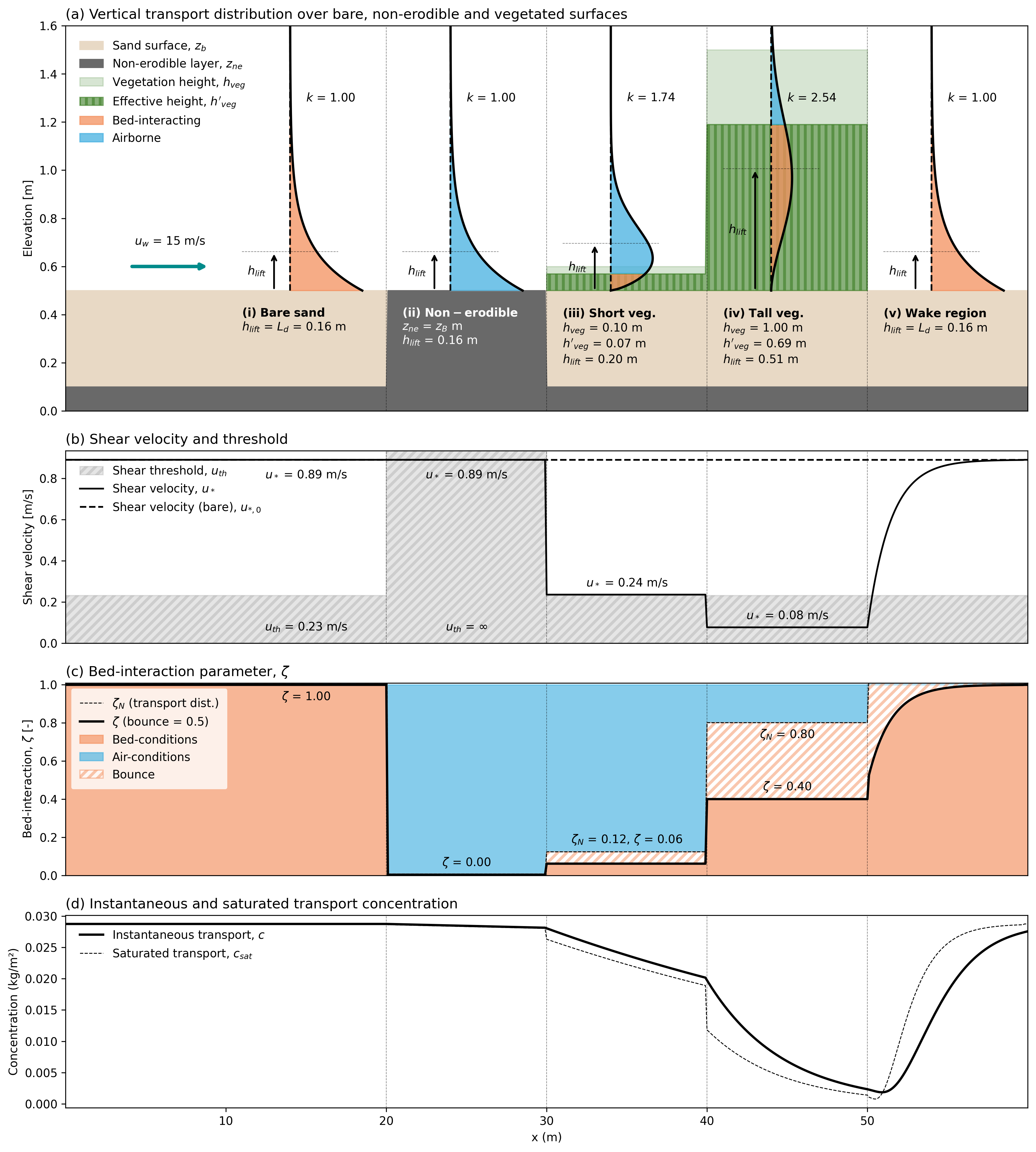
Fig. 9 Vertical transport distribution over bare sand, non-erodible layers, and varying vegetation canopies, illustrating the computation of the bed-interaction parameter \(\zeta\).
The combined saturation concentration \(c_{\mathrm{sat}}\) [\(\mathrm{kg/m^3}\)] is computed as the weighted sum of these two modes:
The dimensionless weights \(w_{\mathrm{air}}\) and \(w_{\mathrm{bed}}\) [\(\mathrm{-}\)] are controlled by the bed-interaction factor \(\zeta\) (zeta) [\(\mathrm{-}\)], which defines the fraction of the flux actively interacting with the bed. The airborne weight scales with the actual sediment concentration \(c\) relative to the airborne carrying capacity:
This formulation simulates transport across different surfaces:
Bare sediment surface (\(\zeta = 1\)): All transport is affected by bed conditions. Bare sand and inundated cells default to 1.
Non-erodible surface (\(\zeta = 0\)): Transport is decoupled from the bed, allowing sediment to bypass the cell without depositing.
Intermediate (\(0 < \zeta < 1\) ): The canopy intercepts a portion of the sediment flux, while the remainder skims over the top.
To estimate \(\zeta\) over vegetation, the model computes the fraction of sediment transport occurring below the effective tiller height \(h'_{\mathrm{veg}}\). A standard flat-bed exponential transport profile concentrates sediment near the bed using a decay length \(L_h\) (where \(L_h = 2 u_*^2/g\)):
Integrating this exponential profile over a canopy yields \(\zeta \approx 1\), failing to reproduce skimming. To reproduce detached, uplifted transport behavior, this is extended to a Weibull distribution:
The extent of the vegetation-induced lift is determined by a lifting coefficient \(\alpha_{\mathrm{lift}}\) (alpha_lift) [\(\mathrm{-}\)] that scales the effective tiller height to define the physical lift height \(h_{\mathrm{lift}}\) [\(\mathrm{m}\)]:
The dimensionless shape parameter \(k\) [\(\mathrm{-}\)] is prescribed as a function of this lift height, utilizing empirical calibration constants \(a_k\) and \(b_k\) [\(\mathrm{-}\)]. For a bare surface, \(h_{\mathrm{lift}} = L_h\), reducing the shape parameter to \(k=1\) (recovering the standard exponential profile):
The Weibull scale parameter \(h_{\mathrm{scale}}\) [\(\mathrm{m}\)] is derived analytically using the standard Gamma function \(\Gamma(z)\) to ensure the bulk transport correctly centers around \(h_{\mathrm{lift}}\):
By integrating this profile up to the effective tiller height \(h'_{\mathrm{veg}}\), the model calculates the raw trapped fraction \(\zeta_0\):
Because sparse vegetation does not cause in “full” skimming, this is adjusted by the relative tiller density using the parameter \(\theta_\zeta\) (theta_zeta) [\(\mathrm{-}\)]:
The final bed-interaction factor accounts for airborne sediment bouncing directly through the canopy using a numerical bounce factor \(b\) (bounce) [\(\mathrm{-}\)]:
Finally, to prevent abrupt deposition in the vegetation wake, the spatial recovery of \(\zeta\) to its non-vegetated base value (\(\zeta = 1\)) is smoothed proportionally to the leeside shear reduction (\(R_{\mathrm{veg}}/R_{0,\mathrm{veg}}\)), ensuring gradual adjustment within the wake region.
Vegetation Mortality
Method duran
Vegetation is subject to destruction caused by hydrodynamic processes. In the event of cell inundation by high water levels, the vegetation density \(\rho_{\text{veg}}\) in the affected grid cells is instantaneously or proportionally reduced to mimic storm-induced erosion of the canopy.
Method grass
Because tiller height and tiller density are fundamentally coupled, changes in one necessitate updates in the other. Mortality and structural changes occur through three primary drivers:
1. Burial and Erosion Dieback: When local burial/erosion rates exceed the plant’s tolerance range, vertical growth becomes negative (\(\partial h_{\text{veg}}/\partial t < 0\)). To represent the physical thinning of the dying patch, the tiller density decays proportionally to the relative loss in height, using a thinning factor \(\gamma_{N_t}\) [\(\mathrm{-}\)]:
2. Recruitment Averaging: When new tillers establish via seed or clonally (\(\partial N_t/\partial t > 0\)), they emerge at the bed surface with an initial height of zero. Therefore, the cell-averaged vegetation height mathematically decreases proportionally:
3. Inundation-driven Decay: Tiller density \(N_t\) decays continuously during inundation events at a rate proportional to the relative water depth \(h_w\) [\(\mathrm{m}\)] (computed as Total Water Level minus bed elevation):
Here, \(T_{\text{flood}}\) (T_flood) [\(\mathrm{s}\)] is the prescribed inundation decay timescale. While this random thinning removes tillers, it does not alter the average height of the surviving canopy.
Hydrodynamics and Surface Moisture
Aeolis computes …. for … and … and …
Water levels, Waves and Run-up
PLACEHOLDER: TWL, SWL, zs, hw, eta, R, …
The runup height and wave setup are computed using the Stockdon formulas [Stockdon et al., 2006]. Their parameterization differs depending on the dynamic beach steepness expressed through the Irribaren number:
where \({H_0}\) is the significant offshore wave height, \({L_0}\) is the deepwater wavelength, and \({\tan \beta}\) is the foreshore slope.
For dissipative conditions, \({\xi}\) < 0.3, the runup, \({R_2}\), is parameterized as,
and wave setup:
For \({\xi}\) > 0.3, runup is paramterized as,
and wave setup:
Surface Moisture
PLACEHOLDER
Hydraulic Sediment Mixing
PLACEHOLDER
Marine-driven Bed Level Change
Bed-level change due to marine-driven dune erosion occurs when the total water level exceeds the base of the dune, or the dune toe elevation (dune_toe_elevation). See dune-erosion for more information.
Groundwater Module (Hallin, 2023)
Wave runup, capillary rise from the beach groundwater, and precipitation periodically wet the intertidal beach temporally increasing the shear velocity threshold ( Fig. 10). Infiltration and evaporation subsequently dry the beach.
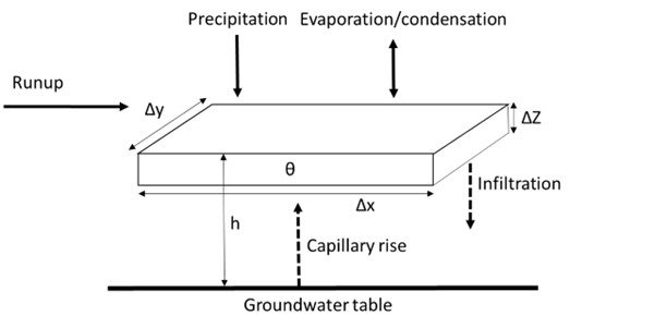
Fig. 10 Illustration of processes influencing the volumetric moisture content \(\theta\) at the beach surface.
The structure of the surface moisture module and included processes are schematized in Fig. 11. The resulting surface moisture is obtained by selecting the largest of the moisture contents computed with the water balance approach (right column) and due to capillary rise from the groundwater table (left column). The method is based on the assumption that the flow of soil water is small compared to the flow of groundwater and that the beach groundwater dynamics primarily is controlled by the water level and wave action at the seaward boundary [Raubenheimer et al., 1999], [Schmutz, 2014]. Thus, there is no feedback between the processes in the right column of Fig. 11 and the groundwater dynamics described in the left column.

Fig. 11 Implementation of surface moisture processes in the AeoLiS.
Groundwater under sandy beaches can be considered as shallow aquifers, with only horizontal groundwater flow so that the pressure distribution is hydrostatic [Baird et al., 1998, Brakenhoff et al., 2019, Nielsen, 1990, Raubenheimer et al., 1999]. The cross-shore flow dominates temporal variations of groundwater levels. Alongshore, groundwater table variations are typically small [Schmutz, 2014]. Although the surface moisture model can be extended over a two-dimensional grid, the groundwater simulations are performed for 1D transects cross-shore to avoid numerical instabilities at the seaward boundary and reduce computational time.
The beach aquifers is schematised as a sandy body, with saturated hydraulic conductivity, \(K\), and effective porosity, \({n_e}\). The aquifer is assumed to rest on an impermeable surface, where \(D\) is the aquifer depth. The groundwater elevation relative to the mean sea level (MSL) is denoted \(\eta\), and the shore-perpendicular x-axis is positive landwards, with an arbitrary starting point. The sand is assumed to be homogenous and isotropic. In this context, isotropy implies that hydraulic conductivity is independent of flow direction.
The horizontal groundwater discharge per unit area, \(u\), is then governed by Darcy’s law,
and the continuity equation (see e.g., [Nielsen, 2009]),
where \(t\) is time.
The groundwater overheight due to runup, \({U_l}\), is computed by [Kang et al., 1994, Nielsen et al., 1988],
where \({C_l}\) is an infiltration coefficient (-), and \(f(x)\) is a function of \(x\) ranging from 0 to 1. \({x_S}\) is the horizontal location of the sum of the still water level and wave setup, and \({x_R}\) is the horizontal location of the runup limit:
Substitution of \(u\) (Equation (75)) in the continuity equation (Equation (76)) with the addition of \({U_l}/{n_e}\) gives the nonlinear Boussinesq equation:
Numerical solution of the Boussinesq groundwater equation
The Boussinesq equation is solved numerically with a central finite difference method in space and a fourth-order Runge-Kutta integration technique in time:
The Runge-Kutta time-stepping, where \(\Delta t\) is the length of the timestep, is defined as,
where, \(i\) is the grid cell in x-direction and \(t\) is the timestep. The central difference solution to \(f(\eta)\) is obtained through discretisation of the Boussinesq equation,
The seaward boundary condition is defined as the still water level plus the wave setup . If the groundwater elevation is larger than the bed elevation, there is a seepage face, and the groundwater elevation is set equal to the bed elevation. On the landward boundary, a no-flow condition, \(\frac{{\partial \eta }}{{\partial t}} = 0\) (Neumann condition), or constant head, \(\eta = constant\) (Dirichlet condition), is prescribed.
Capillary rise
Soil water retention (SWR) functions describe the surface moisture due to capillary transport of water from the groundwater table [van Genuchten, 1980]:
where \(h\) is the groundwater table depth, \(\alpha\) and \(n\) are fitting parameters related to the air entry suction and the pore size distribution. The parameter \(m\) is commonly parameterised as \(m = 1 - 1/n\).
The resulting surface moisture is computed for both drying and wetting conditions, i.e., including the effect of hysteresis. The moisture contents computed with drying and wetting SWR functions are denoted \({\theta ^d}(h)\) and \({\theta ^w}(h)\), respectively. When moving between wetting and drying conditions, the soil moisture content follows an intermediate retention curve called a scanning curve. The drying scanning curves are scaled from the main drying curve and wetting scanning curves from the main wetting curve. The drying scanning curve is then obtained from [Mualem, 1974]:
where \({h_\Delta}\) is the groundwater table depth at the reversal on the wetting curve.
The wetting scanning curve is obtained from [Mualem, 1974]:
where \({h_\Delta}\) is the groundwater table depth at the reversal on the drying curve.
Infiltration
Infiltration is accounted for by assuming that excess water infiltrates until the moisture content reaches field capacity, \({\theta_fc}\). The moisture content at field capacity is the maximum amount of water that the unsaturated zone of soil can hold against the pull of gravity. For sandy soils, the matric potential at this soil moisture condition is around - 1/10 bar. In equilibrium, this potential would be exerted on the soil capillaries at the soil surface when the water table is about 100 cm below the soil surface, \({\theta _{fc}} = {\theta ^d}(100)\).
Infiltration is represented by an exponential decay function that is governed by a drying time scale \(T_{\mathrm{dry}}\). Exploratory model runs of the unsaturated soil with the HYDRUS1D [Šimůnek et al., 1998] hydrology model show that the increase of the volumetric water content to saturation is almost instantaneous with rising tide. The drying of the beach surface through infiltration shows an exponential decay. In order to capture this behavior the volumetric water content is implemented according to:
An alternative formulation is used for simulations that does not account for ground water and SWR processes,
where \(\eta\) [m+MSL] is the instantaneous water level, \(z_{\mathrm{b}}\) [m+MSL] is the local bed elevation, \(p_{\mathrm{V}}^n\) [-] is the volumetric water content in time step \(n\), \(\Delta t^n\) [s] is the model time step and \(\Delta z\) is the bed composition layer thickness. \(T_{\mathrm{dry}}\) [s] is the beach drying time scale, defined as the time in which the beach moisture content halves.
Precipitation and evaporation
A water balance approach accounts for the effect of precipitation and evaporation,
where \(P\) is the precipitation, \(E\) is the evaporation, and \(\Delta z\) is the thickness of the surface layer.
Evaporation is simulated using an adapted version of the Penman-Monteith equation [Shuttleworth, 1993] that is governed by meteorological time series of solar radiation, temperature and humidity.
\(E_{\mathrm{v}}\) [m/s] is the evaporation rate that is implemented through an adapted version of the Penman equation [Shuttleworth, 1993]:
where \(m_{\mathrm{v}}\) [kPa/K] is the slope of the saturation vapor pressure curve, \(R_{\mathrm{n}}\) [\(\mathrm{MJ/m^2/day}\)] is the net radiance, \(\gamma_{\mathrm{v}}\) [kPa/K] is the psychrometric constant, \(u_2\) [m/s] is the wind speed at 2 m above the bed, \(\delta e\) [kPa] is the vapor pressure deficit (related to the relative humidity) and \(\lambda_{\mathrm{v}}\) [MJ/kg] is the latent heat vaporization. To obtain an evaporation rate in [m/s], the original formulation is multiplied by \(9 \cdot 10^7\).
Morphological change
PLACEHOLDER
Bed Level Update
PLACEHOLDER
Avalanching
PLACEHOLDER
Dune Erosion
Wave-driven dune erosion occurs when the TWL exceeds the dune toe elevation (dune_toe_elevation) [m]. The amount of sediment eroded from the dune is dependent on the frequency of collisions with the dune and the exceedenace of the TWL over the dune toe elevation. The volume of eroded sediment is calculated following the Palmsten and Holman (2012) dune erosion formula:
where \(V\) left[ frac{m^3}{m} right] is volume eroded, \(C_s\) is the dune erodibility coefficient, and \(N_c\) is the number of bore collisions. The volume of sediment is removed landward of the dune toe elevation contour and the avalanching process prevents formation of vertial scarps.
Beach Evolution
Beach shape and size contributes to the overall sediment supply available for aeolian sediment transport. AeoLiS includes numerous approaches to represent temporal and spatial variability in sediment supply related to beach evolution (Figure 1a-d). These approaches do not explicitly currently account for wave-driven processes and their role on beach shape and volume changes, however the available methods are meant to mimic realistic expected behaviors and avoid the need to couple model interfaces with external tools. For the purposes of this beach sediment supply function, the shoreline is defined as the seaward boundary of the beach profile (default :math:’xshoreline’ and :math:’zshoreline’ are 0 m; e.g., Figure 1e-f)) and shoreline change rate (:math:’shoreline_change_rate’) is the rate of change at the 0 m contour. Four specific methods, specified in the input file as method_wet_supply, are implemented, as follows below:
``wet_bed_reset``maintains stability of the bed by assuming any beach volume loss from aeolian sediment transport below the maximum wave runup level is replenished by marine processes. This assumption means the inundated beach profile is continuously reset to its initial morphology (Figure 1a). Input dune toe elevation and beach slope are not used in this method.
Note
wet_bed_reset is the default method_wet_supply, while the other methods may only be necessary if modeling a long-term dune evolution case study with high shoreline change rates.
vertical_beach_growth converts a user input horizontal shoreline_change_rate (default 0 m contour) into a vertical beach accretion rate with the following equation:
The vertical_beach_growth method models a linear beach with increased elevation every time step (Figure 1c). The beach maintains a fixed input beach_slope throughout the simulation and has an upper bound of the input dune_toe_elevation (Figure 1g-h). Though this method simulates sediment supply to the dune, it is important to note that over longer simulation time, the beach width is not maintained.
constant_SCR_constant_tanB simulates horizontal and vertical shoreline change using a fixed input beach_slope and fixed input dune_toe_elevation. Like method vertical_beach_growth, constant_SCR_constant_tanB generates a new linear beach profile at each timestep, based on the input beach_slope and upper bounded by the input dune_toe_elevation. However, this method also extends the beach seaward to maintain the beach width throughout the simulation (Figure 1b), resulting in the evolution of both shoreline elevation and position (Figure 1e-f). To use constant_SCR_constant_tanB, it is important to note that the initial input grids must have extra seaward x-domain added to allow the beach to prograde.
constant_SCR_variable_tanB simulates horizontal shoreline change while allowing the beach_slope to evolve with the shoreline position and dune toe elevation to vary slightly with the upper bound of the input dune_toe_elevation (Figure 1d-h). A new beach slope is calculated and used to generate a linear beach each timestep. Similar to the constant_SCR_constant_tanB, the x-domain of the input files must be extended seaward to implement this method. This method simulates more natural beach and dune evolution than the other methods available.
